FEgrow: An Open-Source Molecular Builder and Free Energy Preparation Workflow
Authors: Mateusz K Bieniek, Ben Cree, Rachael Pirie, Joshua T. Horton, Natalie J. Tatum, Daniel J. Cole
Add chemical functional groups (R-groups) in user-defined positions
Output ADMET properties
Perform constrained optimisation
Score poses
Output structures for free energy calculations
Overview
This notebook demonstrates the entire FEgrow workflow for generating
a series of ligands with a common core for a specific binding site, via
the addition of a user-defined set of R-groups.
These de novo ligands are then subjected to ADMET analysis. Valid conformers of the added R-groups are enumerated, and optimised in the context of the receptor binding pocket, optionally using hybrid machine learning / molecular mechanics potentials (ML/MM).
An ensemble of low energy conformers is generated for each ligand, and
scored using the gnina convolutional neural network (CNN). Output
structures are saved as pdb files ready for use in free energy
calculations.
The target for this tutorial is the main protease (Mpro) of SARS-CoV-2, and the core and receptor structures are taken from a recent study by Jorgensen & co-workers.
import prody
from rdkit import Chem

import fegrow
from fegrow import RGroups, RLinkers
Prepare the ligand template
The provided core structure lig.pdb has been extracted from a
crystal structure of Mpro in complex with compound 4 from the
Jorgensen study (PDB: 7L10), and a Cl atom has been removed to allow
growth into the S3/S4 pocket. The template structure of the ligand is
protonated with Open Babel:
!obabel sarscov2/lig.pdb -O sarscov2/coreh.sdf -p 7
1 molecule converted
Load the protonated ligand into FEgrow:
init_mol = Chem.SDMolSupplier('sarscov2/coreh.sdf', removeHs=False)[0]

# get the FEgrow representation of the rdkit Mol
template = fegrow.RMol(init_mol)
Show the 2D (with indices) representation of the core. This is used to select the desired growth vector.
template.rep2D(idx=True, size=(500, 500))
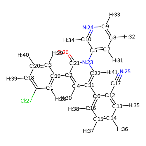
Using the 2D drawing, select an index for the growth vector. Note that it is currently only possible to grow from hydrogen atom positions. In this case, we are selecting the hydrogen atom labelled H:40 to enable growth into the S3/S4 pocket of Mpro.
attachment_index = [40]
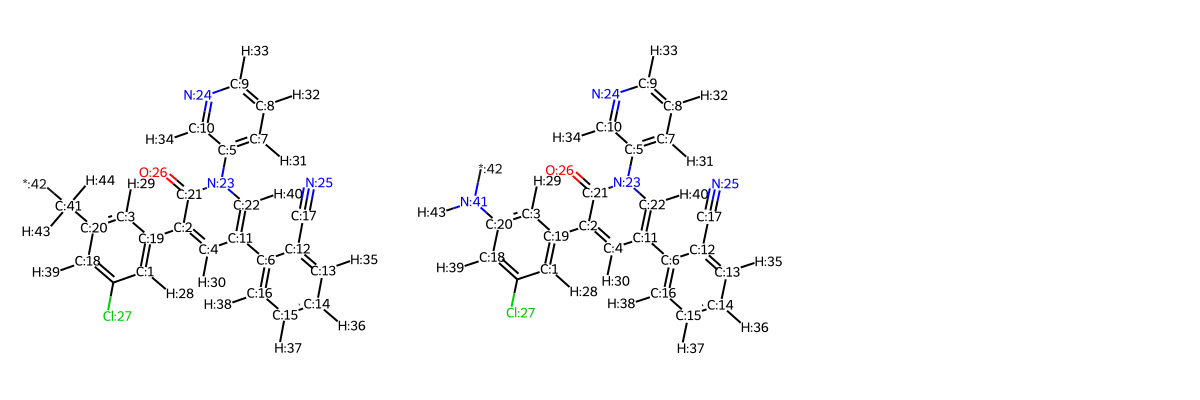
Optional: insert a linker
We have added a library of linkers suggested by Ertl et al. If you wish to extend your R groups selection via a linker, select them below. :1 is defined to be attached to the core (there exists a mirror image of each linker i.e. :1 & *:2 swapped).
Linkers combinatorially augment chosen R groups, so if you choose 2 linkers and 3 R groups, this will result in 6 molecules being built.
RLinkers
# get linkers programmatically
df = RLinkers.dataframe
api_linkers = [ df.loc[df['Name']=='R1CR2']['Mol'].values[0], df.loc[df['Name']=='R1NR2']['Mol'].values[0] ]

# or pick linkers from the grid
grid_linkers = RLinkers.get_selected()

# use grid linkers
linkers = grid_linkers + api_linkers

# create just one template merged with a linker
templates_with_linkers = fegrow.build_molecules(template, linkers, attachment_index)

# visualise:
# note that the linker leaves the second attachement point prespecified (* character)
templates_with_linkers.rep2D(idx=True, size=(500, 500))
Rgroup atom index <rdkit.Chem.rdchem.QueryAtom object at 0x7f4e74146080> neighbouring <rdkit.Chem.rdchem.Atom object at 0x7f4e7091c6a0>
Rgroup atom index <rdkit.Chem.rdchem.QueryAtom object at 0x7f4e7091ca00> neighbouring <rdkit.Chem.rdchem.Atom object at 0x7f4e7091c8e0>
Select RGroups for your template
R-groups can be selected interactively or programmaticaly.
We have provided a set of common R-groups (see
fegrow/data/rgroups/library), which can be browsed and selected
interactively below.
Molecules from the library can alternatively be selected by name, as demonstrated below.
Finally, user-defined R-groups may be provided as .mol files. In
this case, the hydrogen atom selected for attachment should be replaced
by the element symbol R. See the directory manual_rgroups for
examples.
RGroups
# retrieve the interactively selected groups
interactive_rgroups = RGroups.get_selected()

# you can also directly access the built-in dataframe programmatically
groups = RGroups.dataframe
R_group_ethanol = groups.loc[groups['Name']=='*CCO']['Mol'].values[0]
R_group_cyclopropane = groups.loc[groups['Name'] == '*C1CC1' ]['Mol'].values[0]

# add your own R-groups files
R_group_propanol = Chem.MolFromMolFile('manual_rgroups/propan-1-ol-r.mol', removeHs=False)

# make a list of R-group molecule
selected_rgroups = [R_group_propanol, R_group_ethanol, R_group_cyclopropane] + interactive_rgroups
selected_rgroups
[<rdkit.Chem.rdchem.Mol at 0x7f4e74105420>,
 <rdkit.Chem.rdchem.Mol at 0x7f4e98be2560>,
 <rdkit.Chem.rdchem.Mol at 0x7f4e98ba9de0>]
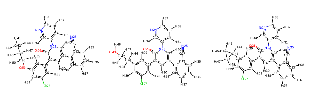
Build a congeneric series
Now that the R-groups have been selected, we merge them with the ligand core:
# we can either use the original template (so no linker)
# in this case we have to specify the attachment index
rmols = fegrow.build_molecules(template, selected_rgroups, attachment_index)

# or we can use the template merged with the linker
# in which case the attachement point is not needed (R* atom is used)
# rmols = fegrow.build_molecules(templates_with_linkers, selected_rgroups)
Rgroup atom index <rdkit.Chem.rdchem.QueryAtom object at 0x7f4e70970640> neighbouring <rdkit.Chem.rdchem.Atom object at 0x7f4e70970160>
Rgroup atom index <rdkit.Chem.rdchem.QueryAtom object at 0x7f4e70970280> neighbouring <rdkit.Chem.rdchem.Atom object at 0x7f4e70970be0>
Rgroup atom index <rdkit.Chem.rdchem.QueryAtom object at 0x7f4e70970640> neighbouring <rdkit.Chem.rdchem.Atom object at 0x7f4e70970c40>
rmols
| Smiles | Molecule | |
|---|---|---|
| ID | ||
| 0 | [H]c1nc([H])c(-n2c([H])c(-c3c([H])c([H])c([H])... |  |
| 1 | [H]OC([H])([H])C([H])([H])c1c([H])c(Cl)c([H])c... |  |
| 2 | [H]c1nc([H])c(-n2c([H])c(-c3c([H])c([H])c([H])... |  |
The R-group library can also be viewed as a 2D grid, or individual molecules can be selected for 3D view (note that the conformation of the R-group has not yet been optimised):
rmols.rep2D()
rmols[0].rep3D()
You appear to be running in JupyterLab (or JavaScript failed to load for some other reason). You need to install the 3dmol extension:
jupyter labextension install jupyterlab_3dmol
<py3Dmol.view at 0x7f4e70932020>
Once the ligands have been generated, they can be assessed for various ADMET properties, including Lipinksi rule of 5 properties, the presence of unwanted substructures or problematic functional groups, and synthetic accessibility.
rmols.toxicity()
| MW | HBA | HBD | LogP | Pass_Ro5 | has_pains | has_unwanted_subs | has_prob_fgs | synthetic_accessibility | Smiles | Molecule | |
|---|---|---|---|---|---|---|---|---|---|---|---|
| ID | |||||||||||
| 0 | 441.918 | 5 | 0 | 5.880 | True | False | False | True | 7.634562 | [H]c1nc([H])c(-n2c([H])c(-c3c([H])c([H])c([H])... | |
| 1 | 427.891 | 5 | 1 | 4.626 | True | False | False | True | 7.501563 | [H]OC([H])([H])C([H])([H])c1c([H])c(Cl)c([H])c... | |
| 2 | 423.903 | 4 | 0 | 5.969 | True | False | False | True | 7.482970 | [H]c1nc([H])c(-n2c([H])c(-c3c([H])c([H])c([H])... | |
For each ligand, a specified number of conformers (num_conf) is
generated by using the RDKit ETKDG
algorithm. Conformers that
are too similar to an existing structure are discarded. Empirically, we
have found that num_conf=200 gives an exhaustive search, and
num_conf=50 gives a reasonable, fast search, in most cases.
If required, a third argument can be added flexible=[0,1,...], which
provides a list of additional atoms in the core that are allowed to be
flexible. This is useful, for example, if growing from a methyl group
and you would like the added R-group to freely rotate.
rmols.generate_conformers(num_conf=50,
                          minimum_conf_rms=0.5,
                          # flexible=[3, 18, 20])
                        )
RMol index 0
Removed 25 duplicated conformations, leaving 26 in total.
RMol index 1
Removed 41 duplicated conformations, leaving 10 in total.
RMol index 2
Removed 40 duplicated conformations, leaving 11 in total.
The protein-ligand complex structure is downloaded, and PDBFixer is used to protonate the protein, and perform other simple repair:
# get the protein-ligand complex structure
!wget -nc https://files.rcsb.org/download/7L10.pdb

# load the complex with the ligand
sys = prody.parsePDB('7L10.pdb')

# remove any unwanted molecules
rec = sys.select('not (nucleic or hetatm or water)')

# save the processed protein
prody.writePDB('rec.pdb', rec)

# fix the receptor file (missing residues, protonation, etc)
fegrow.fix_receptor("rec.pdb", "rec_final.pdb")

# load back into prody
rec_final = prody.parsePDB("rec_final.pdb")
File ‘7L10.pdb’ already there; not retrieving.
@> 2609 atoms and 1 coordinate set(s) were parsed in 0.05s.
@> 4638 atoms and 1 coordinate set(s) were parsed in 0.03s.
View enumerated conformers in complex with protein:
rmols[0].rep3D(prody=rec_final)
You appear to be running in JupyterLab (or JavaScript failed to load for some other reason). You need to install the 3dmol extension:
jupyter labextension install jupyterlab_3dmol
<py3Dmol.view at 0x7f4e709308e0>
Any conformers that clash with the protein (any atom-atom distance less than 1 Angstrom), are removed.
rmols.remove_clashing_confs(rec_final)
RMol index 0
Clash with the protein. Removing conformer id: 25
Clash with the protein. Removing conformer id: 22
Clash with the protein. Removing conformer id: 20
Clash with the protein. Removing conformer id: 14
Clash with the protein. Removing conformer id: 11
Clash with the protein. Removing conformer id: 8
Clash with the protein. Removing conformer id: 7
Clash with the protein. Removing conformer id: 6
Clash with the protein. Removing conformer id: 5
Clash with the protein. Removing conformer id: 4
Clash with the protein. Removing conformer id: 3
RMol index 1
Clash with the protein. Removing conformer id: 2
Clash with the protein. Removing conformer id: 0
RMol index 2
rmols[0].rep3D(prody=rec_final)
You appear to be running in JupyterLab (or JavaScript failed to load for some other reason). You need to install the 3dmol extension:
jupyter labextension install jupyterlab_3dmol
<py3Dmol.view at 0x7f4e7096db70>
The remaining conformers are optimised using hybrid machine learning / molecular mechanics (ML/MM), using the ANI2x neural nework potential for the ligand energetics (as long as it contains only the atoms H, C, N, O, F, S, Cl). Note that the Open Force Field Parsley force field is used for intermolecular interactions with the receptor.
sigma_scale_factor: is used to scale the Lennard-Jones radii of the
atoms.
relative_permittivity: is used to scale the electrostatic
interactions with the protein.
water_model: can be used to set the force field for any water
molecules present in the binding site.
# opt_mol, energies
energies = rmols.optimise_in_receptor(
    receptor_file="rec_final.pdb",
    ligand_force_field="openff",
    use_ani=True,
    sigma_scale_factor=0.8,
    relative_permittivity=4,
    water_model = None
)
RMol index 0
using ani2x
/home/dresio/software/mambaforge/envs/fegrow/lib/python3.10/site-packages/torchani/__init__.py:55: UserWarning: Dependency not satisfied, torchani.ase will not be available
  warnings.warn("Dependency not satisfied, torchani.ase will not be available")
/home/dresio/software/mambaforge/envs/fegrow/lib/python3.10/site-packages/torchani/resources/
failed to equip nnpops with error: No module named 'NNPOps'
Optimising conformer: 100%|█████████████████████| 15/15 [00:15<00:00, 1.02s/it]
RMol index 1
using ani2x
/home/dresio/software/mambaforge/envs/fegrow/lib/python3.10/site-packages/torchani/resources/
failed to equip nnpops with error: No module named 'NNPOps'
Optimising conformer: 100%|███████████████████████| 8/8 [00:07<00:00, 1.04it/s]
RMol index 2
using ani2x
/home/dresio/software/mambaforge/envs/fegrow/lib/python3.10/site-packages/torchani/resources/
failed to equip nnpops with error: No module named 'NNPOps'
Optimising conformer: 100%|█████████████████████| 11/11 [00:08<00:00, 1.33it/s]
Any of the rmols that have no available conformers (due to unresolvable
steric clashes with the protein) can be discarded using the
.discard_missing() function. This function also returns a list of
the indices that were removed, which can be helpful when carrying out
data analysis.
missing_ids = rmols.discard_missing()
Optionally, display the final optimised conformers. Note that, unlike classical force fields, ANI allows bond breaking. You may occasionally see ligands with distorted structures and very long bonds, but in our experience these are rarely amongst the low energy structures and can be ignored.
Conformers are now sorted by energy, only retaining those within 5 kcal/mol of the lowest energy structure:
final_energies = rmols.sort_conformers(energy_range=5)
RMol index 0
RMol index 1
RMol index 2
rmols[0].rep3D()
You appear to be running in JupyterLab (or JavaScript failed to load for some other reason). You need to install the 3dmol extension:
jupyter labextension install jupyterlab_3dmol
<py3Dmol.view at 0x7f4e61282ce0>
Save all of the lowest energy conformers to files and print the sorted energies in kcal/mol (shifted so that the lowest energy conformer is zero).
for i, rmol in enumerate(rmols):
    rmol.to_file(f"best_conformers{i}.pdb")
print(final_energies)
                Energy
ID Conformer
0  0          0.000000
   1          0.000292
   2          0.130588
   3          0.508776
   4          0.509229
   5          1.114966
   6          1.970927
   7          1.972700
   8          2.398551
   9          2.399397
   10         2.406501
   11         2.787855
1  0          0.000000
   1          2.648491
   2          3.030201
   3          4.021199
2  0          0.000000
   1          0.000108
   2          0.000180
   3          0.181695
   4          0.181838
   5          0.181906
   6          0.201162
   7          1.776589
   8          1.776619
   9          1.776679
   10         1.778395
The conformers are scored using the Gnina molecular docking program and convolutional neural network scoring function. [Note that this step is not supported on macOS]. If unavailable, the Gnina executable is downloaded during the first time it is used. The CNNscores may also be converted to predicted IC50 (nM) (see column “CNNaffinity->IC50s”).
affinities = rmols.gnina(receptor_file="rec_final.pdb")
affinities
RMol index 0
RMol index 1
RMol index 2
| CNNaffinity | CNNaffinity->IC50s | ||
|---|---|---|---|
| ID | Conformer | ||
| 0 | 0 | 7.05511 | 88.082575 |
| 1 | 7.05513 | 88.078518 | |
| 2 | 6.82962 | 148.040315 | |
| 3 | 7.08356 | 82.497350 | |
| 4 | 7.08356 | 82.497350 | |
| 5 | 7.01775 | 95.995307 | |
| 6 | 6.79818 | 159.154895 | |
| 7 | 6.79813 | 159.173219 | |
| 8 | 6.69786 | 200.511830 | |
| 9 | 6.69799 | 200.451818 | |
| 10 | 6.58795 | 258.255750 | |
| 11 | 6.85830 | 138.579822 | |
| 1 | 0 | 6.57308 | 267.251407 |
| 1 | 6.67290 | 212.373341 | |
| 2 | 6.73439 | 184.335932 | |
| 3 | 6.52578 | 298.002563 | |
| 2 | 0 | 6.86908 | 135.182353 |
| 1 | 6.86911 | 135.173015 | |
| 2 | 6.86918 | 135.151229 | |
| 3 | 6.72789 | 187.115601 | |
| 4 | 6.72768 | 187.206102 | |
| 5 | 6.72774 | 187.180240 | |
| 6 | 6.26276 | 546.059541 | |
| 7 | 6.91413 | 121.862477 | |
| 8 | 6.91413 | 121.862477 | |
| 9 | 6.91410 | 121.870895 | |
| 10 | 6.91403 | 121.890540 |
Predicted binding affinities may be further refined using the structures
output by FEgrow, using your favourite free energy calculation
engine. See our paper for an example using
SOMD to calculate the relative
binding free energies of 13 Mpro inhibitors.